
Partitions and the Bloch-Okounkov Theorem
Published:
In this post I will briefly explain what is a partition of a positive integer and how it is possible to relate this theory to quasimodular forms via the Bloch-Okounkov theorem.
Partitions
In mathematics, a partition of a number \(n\) is simply a finite sequence of integers \(\lambda_1, \lambda_2, \ldots, \lambda_m\) such that \(\lambda_i \geq \lambda_{i+1}\) and
\[n = \lambda_1 + \lambda_2 + \cdots + \lambda_m,\quad m\geq 1.\]Equivalently, a partition is a sequence of integers \(\lambda = (\lambda_1, \lambda_2, \ldots, \lambda_i, \ldots)\) such that \(\lambda_i \geq \lambda_{i+1}\) and \(\lambda_i = 0\) for all but finitely many indices \(i\). We denote by \(\vert \lambda \vert\) the sum of its entries: \(\vert \lambda \vert = \lambda_1 + \cdots + \lambda_m\).
For example, \((5,3,2)\) is a partition of the number \(10\) and \((3,1,1)\) is a partition of the number \(5\).
Exercise. Find all the seven partitions of the number \(5\).
We will denotes by \(\mathcal{P}\) the set of all partitions. For our purpose, we will be working with function \(f : \mathcal{P} \rightarrow \mathbb{Q}\). An example of such function is \(f(\lambda) = \vert \lambda \vert\). Given a function \(f\) defined over \(\mathcal{P}\), it is possible to construct a \(q\)-power series via the \(q\)-bracket:
\[\langle f \rangle_q := \frac{\sum_{\lambda \in \mathcal{P}} f(\lambda) q^{\vert \lambda \vert}}{\sum_{\lambda \in \mathcal{P}}q^{\vert \lambda \vert}} \in \mathbb{Q}[[q]].\]The theorem of Bloch and Okounkov asserts that this \(q\)-bracket correspond to the \(q\)-expansion of a quasimodular form for a certain class of functions \(f:\mathcal{P} \rightarrow \mathbb{Q}\) (called shifted symmetric polynomials). To defines these shifted symmetric polynomials, we will need the notion of Young diagram and the Frobenius coordinates of a partition.
Young Diagrams and Frobenius Coordinates
One way of representing a partition visually is by the use of Young diagrams. The Young diagram of a partition \(\lambda = (\lambda_1, \ldots, \lambda_m)\) is given by a series of squares:
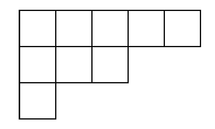
In the example above, the top row of squares correspond to \(\lambda_1 = 5\), the second row correspond \(\lambda_2 = 3\) and so on.
Exercise. Draw the Young diagram of \((5,4,3,3,2,1)\).
Now, using the Young diagram of a partition, it is now possible to define the Frobenius coordinates of a partition. Let \(\lambda\) be a partition. The Frobenius coordinates of \(\lambda\) is the numbers
\[(r; a_1, a_2, \ldots, a_r; b_1, b_2, \ldots, b_r)\]such that
- \(r\) is the length of the longest principal diagonal in the Young diagram of \(\lambda\);
- \(a_1 > \ldots > a_i >\ldots > a_r \geq 0\) are the number of cells to the right of the \(i\)-th cell of this diagonal;
- \(b_1 > \ldots > b_i> \ldots > b_r \geq 0\) are the number of cells below the \(i\)-th cell of this diagonal.
There is nothing better than an example to illustrate this definition. Consider the partition \(\lambda = (5, 3, 1)\) with Young diagram:
By drawing the longest principal diagonal and counting the number of cells we get:
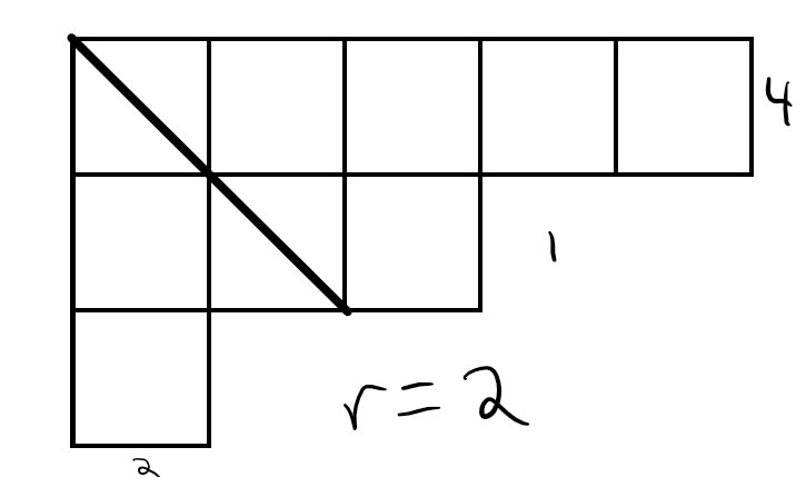
Thus, the Frobenius coordinates of \(\lambda = (5, 3, 1)\) is
\[(2; 4, 1; 2; 0)\]Exercise. Find the Frobenius coordinates of \(\lambda = (5,5,4,1)\).
Shifted Symmetric Polynomials
In this section, I will give a brief overview of the shifted symmetric polynomials. First, we need to define two invariants of a partition: \(P_k(\lambda)\) and \(Q_k(\lambda)\) for an integer \(k\geq 0\).
Definition. Let \(\lambda\) be a partition with Frobenius coordinates \((r; a_1, \ldots, a_r; b_1,\ldots, b_r)\) we define
\[P_k(\lambda) := \sum_{i = 1}^r \left[ (a_i + 1/2)^k - (-b_i - 1/2)^k \right], \quad k\geq 0;\] \[Q_k(\lambda) := \frac{P_{k-1}(\lambda)}{(k-1)!} + \beta_k,\quad k\geq 1;\]where \(\beta_k\) is the \(k\)-th coefficients of the expansion of \(\frac{z/2}{\mathrm{sinh(z/2)}}\) around \(z=0\).
Definition. A shifted symmetric polynomial is a function \(f:\mathcal{P} \rightarrow \mathbb{Q}\) living in \(\mathcal{R} := \mathbb{Q}[Q_1, Q_2, \ldots, Q_k, \ldots]\). We define \(\mathcal{R}_k \subset \mathcal{R}\) to be the weight \(k\) graded component of \(\mathcal{R}\), that is the subring generated by the weight \(k\) homogenenous monomials:
\[\mathcal{R}_k = \langle Q_{k_1}^{m_1}\cdots Q_{k_N}^{m_N} : k_i, m_i\geq 1, k_1 m_1 + \cdots + k_N m_N = k \rangle\]Theorem (Bloch-Okounkov). For any \(f\in \mathcal{R}_k\), the \(q\)-bracket \(\langle f \rangle_q\) correspond to the \(q\)-expansion of a quasimodular forms of weight \(k\) for \(\mathrm{SL}_2(\mathbb{Z})\).
This theorem is interesting as it relates two apparently different concept: partitions and (quasi)modular forms. In particular, the Bloch-Okounkov theorem can be seen as a tool for studying partitions via quasimodular forms and vice versa.
A proof of this theorem can be found in the the main reference for this post:
Don Zagier, Partitions, quasimodular forms and the Bloch-Okounkov theorem
In the next weeks, I will be working on the SageMath implementation of the objects described above. In a later version of Sage, it should be possible to do computations with quasimodular forms and to compute the \(q\)-bracket of a shifted symmetric polynomial.
Thanks for reading!